Study Analysis
Follow these steps to Create a New Analysis Report:
Step 1: Select the Study
After logging into Q Method Software, click on the title of the study in the Study List interface. This brings you to the Study Dashboard and populates the study's sub-navigation.
Step 2: View Study Analysis Reports
On the left side study sub-navigation, click Study Analysis to view the analysis interfaces for the study.
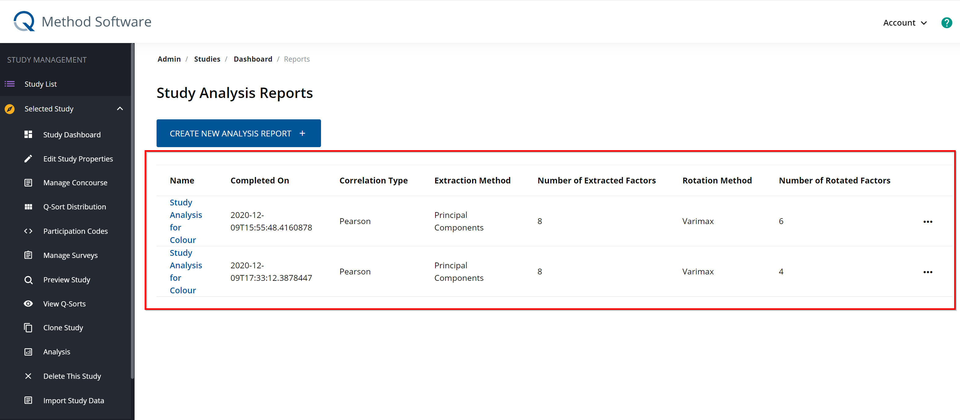
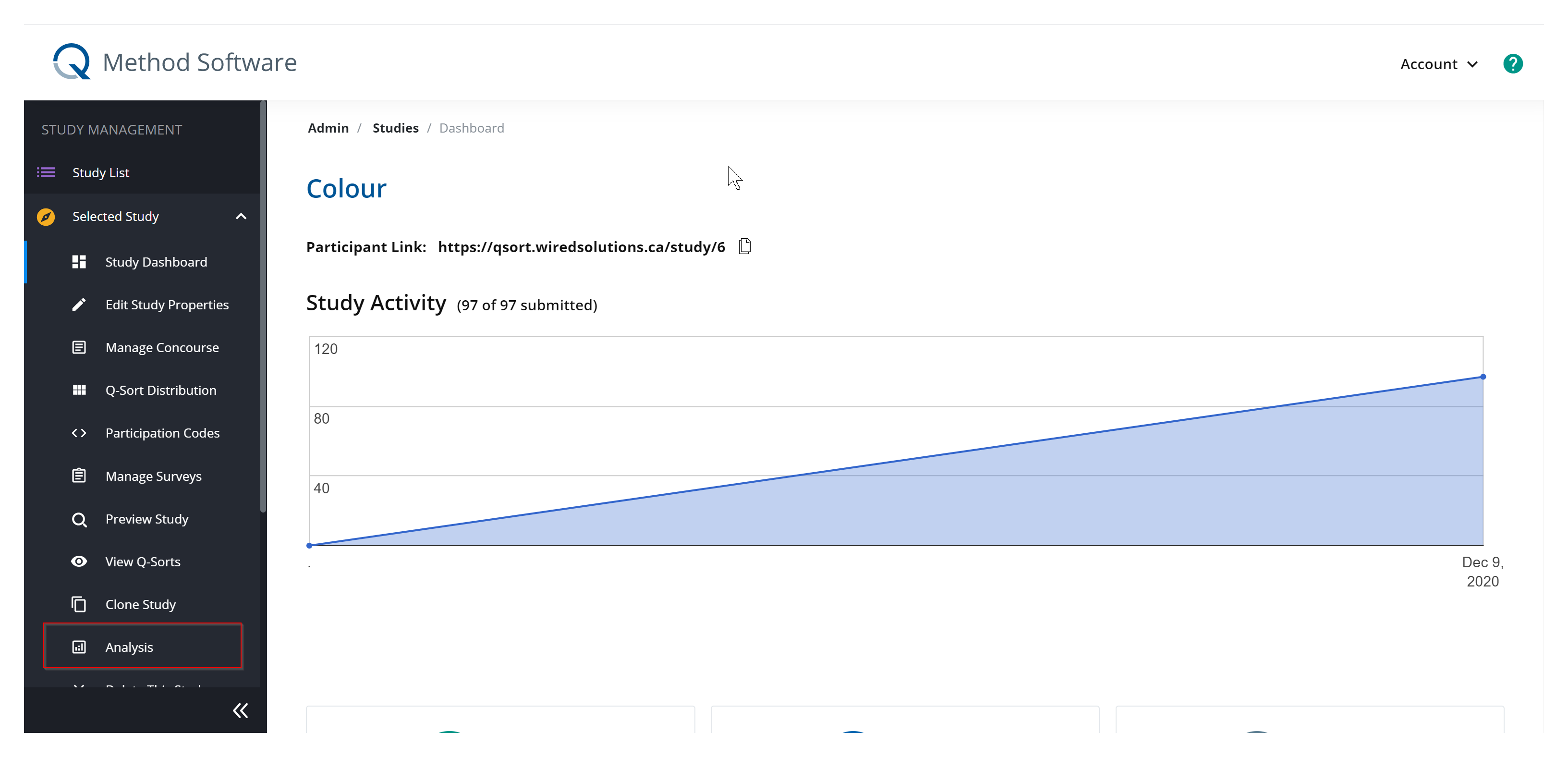 This will bring you to the Study Analysis Reports interface that lists all previously created analysis reports.
Tip
You can create multiple different reports based on different analysis methods.
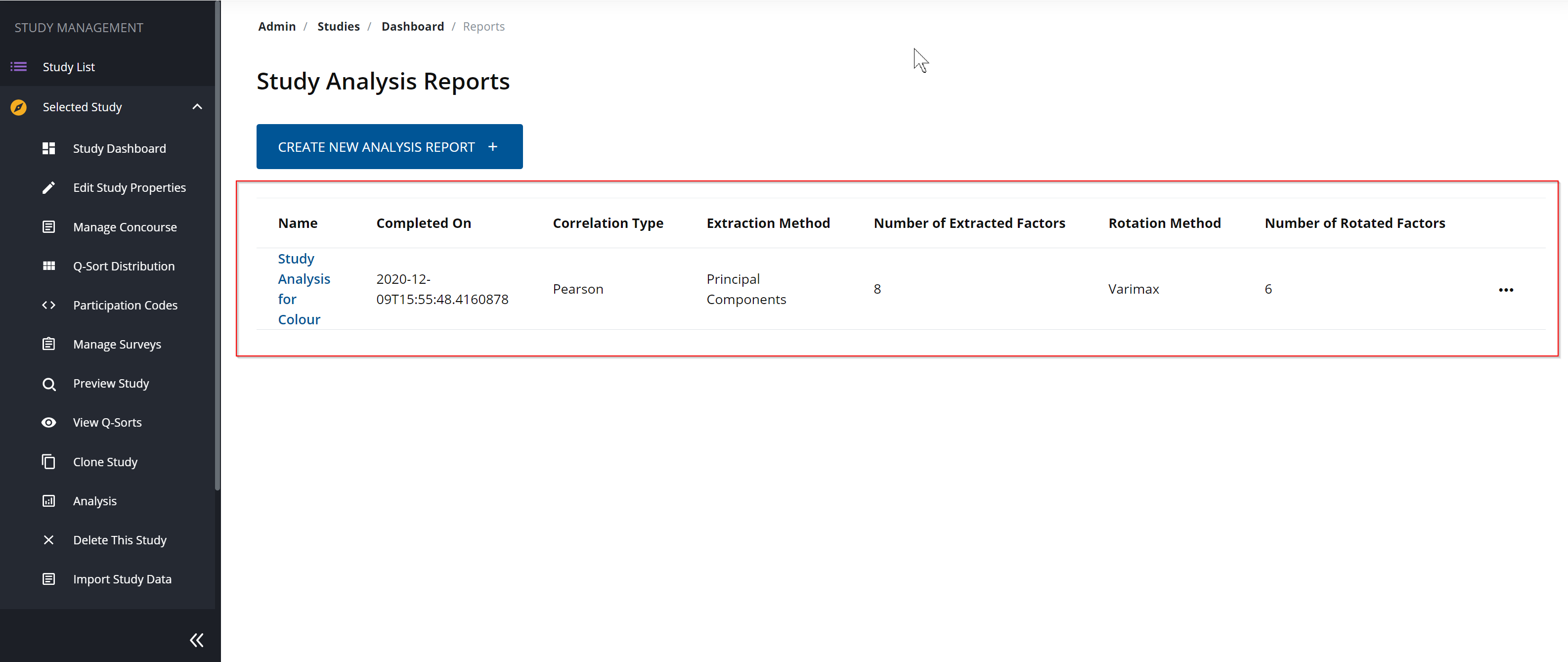
Each saved report may contain different configurations or settings for the same study (i.e. one report might employ a Principal Component Analysis with Varimax Rotation, and another report might employ a Centroid Analysis with Hand Rotation). The details of each report can be found in this table as shown below:
Warning
Only the saved analysis reports will show up here.
Step 3: Create New Analysis Report
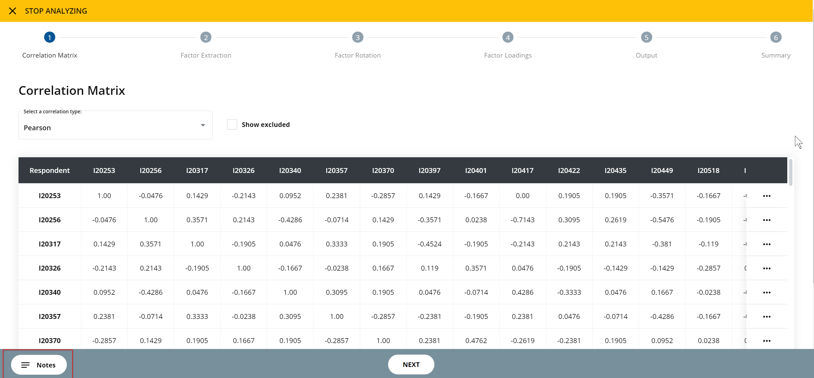
To create a new analysis report, click the create new analysis report button. A six-step process will be displayed to complete the analysis report.
Notes
In the bottom left-hand corner, you will see a notes button. You can write any notes here that you might need for various purposes throughout the analysis.
To complete the analysis report, follow these steps:
Step 3.1: Choose your correlation matrix
Select a correlation type by clicking on the drop-down menu. You can choose either Pearson or Spearman. Pearson correlation is a standardized measure of linear association between two sets of scores, and Spearman correlation is a standardized measure of the linear association between two sets of ranked scores.
Once you have selected a correlation type, the table will update in real-time to display the correlation matrix. You may decide to exclude, delete, or view particular q-sorts at this stage. To do this, click the menu option located at the end of the row of the specific q-sort.
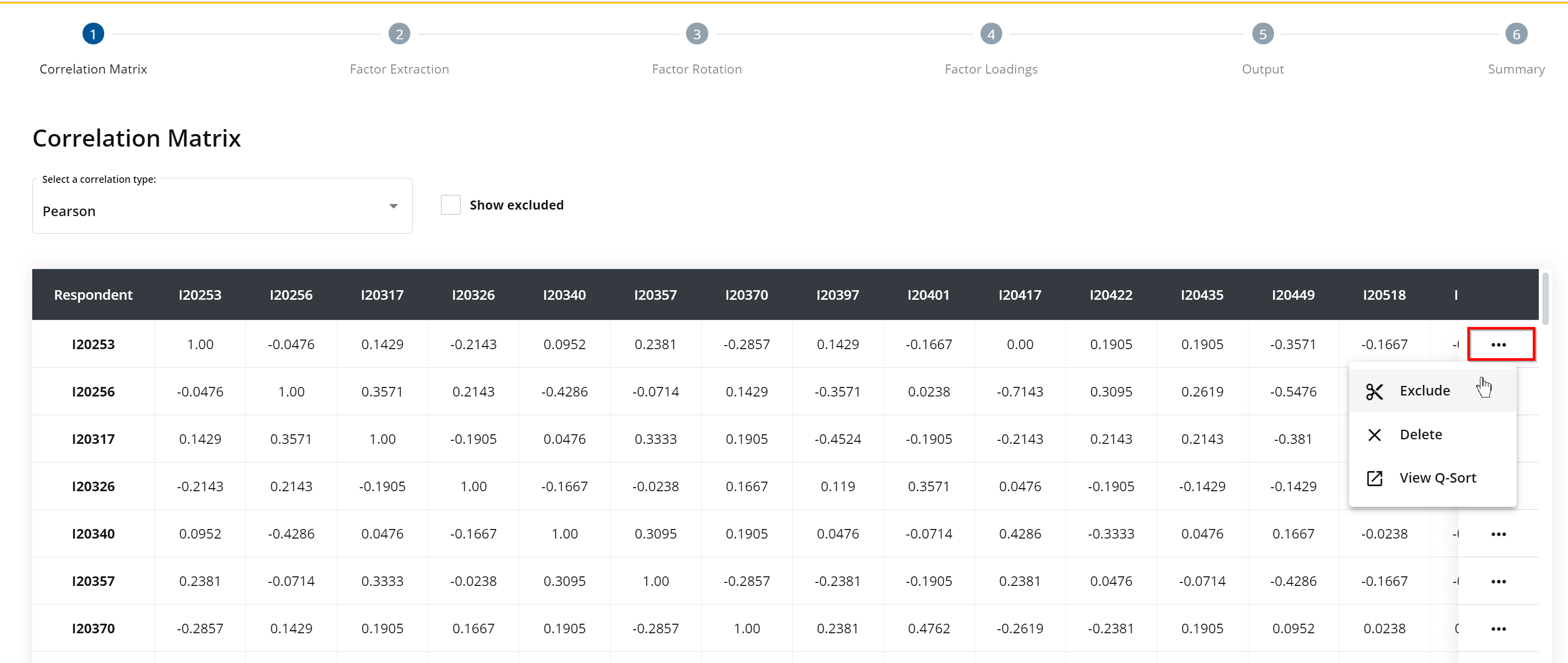
You may decide to show any excluded data in your report. To do this, check the show excluded box above the correlation matrix.
Click Next to continue to step 2.
Step 3.2: Factor Extraction
The next step is to pick a method of factor extraction. The goal of factor extraction is to find repeated patterns in the data, and this can be achieved with Principal Component Analysis or Centroid Analysis.
Principal Component (PCA) is a data condensation technique that is used when factors are orthogonal to each other, thus being statistically and linearly independent of one another. PCA allows you to combine your predictors and drop the eigenvectors that are relatively unimportant. PCA provides researchers with a more structured analysis, which includes:
- A measure of how each variable is associated with one another (covariance matrix)
- The directions in which our data are dispersed (eigenvectors)
- The relative importance of these different directions (eigenvalues)
Centroid Extraction (CE) is commonly used when research is based on a priori hypotheses; it extracts the largest sum of absolute loadings for each factor. CE, paired with varimax rotation (more on this later), is often used for journal publications. In CE, a component is being extracted and it draws attention to shared variance, unique variance, and error variance.
To conduct a Principal Component Analysis, follow these steps:
Select Principal Component Extraction. Unlike Centroid Analysis, the number of factors will automatically be chosen and reflected in the “extracted factors” table.
The Extracted Factors table will update in real-time, which displays the unrotated factor loadings of all q-sorts. Every q-sort will have a loading on every factor, which are expressed as correlation coefficients (i.e. +/- 0.81). The greater the number, the stronger the association; likewise, the smaller the number, the weaker the association.
To determine whether the factor loadings are significant, you may follow the steps as demonstrated below:
A significant factor loading at the 0.01 level can be calculated using the following equation: 2.58 x (1 ÷ √No. of items in qset)
A significant factor loading at the 0.05 level can be calculated using the following equation: 1.96 (1÷ √No. of items in qset)
For example, imagine that your study contains 43 q-sets. If you are working at the 0.01 level, you would complete the following steps:
2.58 x (1 ÷ √No. of items in qset)
2.58 x (1 ÷ √ 43 )
2.58 x (1 ÷ 6.56)
2.58 x 0.15
= +/- 0.39Therefore, you need a factor loading of +/- 0.39 at the 0.01 level for it to be considered a significant correlation. This coefficient (+/- 0.39) allows you to identify which factor each q-sort loads onto significantly.
At this point in the process, you should be thinking about which factors you want to retain for rotation and analysis (which takes place in step 3). We have included an Additional Information tab and a Scree Plot tab to help with your decision.
The Additional Information tab is designed to apply the Kaiser-Guttman Criterion and Humphrey’s Rule to each factor, which can help guide your factor retention process.
The Additional Information tab displays:- the eigenvalue
- the % explained variance
- the cumulative variance
- Humphrey’s Rule (the cross-product of the factor’s two highest factor loadings)
- Standard error
You may choose to apply the Kaiser-Guttman Criterion and/or Humphrey’s Rule to the data set.
- The Kaiser-Guttman Criterion states that factors should be retained if they have an eigenvalue greater than 1.00. You can either look at the eigenvalues of all the factors, or simply press the Apply Kaiser-Guttman Criterion button. This will automatically highlight all the factors that satisfy this criterion.
- Humphrey’s Rule states that factors should be retained if the cross-product of the two highest factor loadings exceeds twice the standard error. This interface automatically determines the cross-product of the two highest factor loadings for each factor, which is displayed under Humphrey’s Rule in the table. You can press the Apply Humphrey’s Rule button, which will automatically highlight the factors that satisfy the criterion.

You may also reference the Scree Plot tab, which displays the eigenvalues (on the y-axis) and the number of factors (on the x-axis) in a downward curve. A scree plot allows you to clearly see where the slope of the curve levels off, which can help you decide which factors to retain for analysis.

You can run a parallel analysis with either random data or study data. A parallel analysis generates data based on the same number of statements, participants, and q-sorts. You will have to do this if you run a PCA.
- To run a parallel analysis, click either Random Data or Study Data. You will see a table that displays the Actual EV, the Mean EV, and the 95th Percentile EV. If the 95th Percentile EV is less than the Actual EV, then the factor should be retained for rotation. A parallel analysis tells you which factors are an acceptable solution.
After you have made note of the factors that you want to retain, click next to continue to step 3.
To conduct a Centroid Analysis, follow these steps:
Select Centroid Extraction.
Select the numbers of factors to extract. This can be done in a few different ways:
- You may arbitrarily choose how many factors to display. If you want to produce a q-sort that represents two dimensions, you may decide to choose only two factors.
- You may also decide to calculate the proportion of variance explained.
- You can include one factor for every 7 or 8 q-sorts (i.e. a study with 40 q-sorts might include 5 factors in a centroid analysis).
- You may look at the provided scree plot, which sorts factors by proportion of variance explained and plots the cumulative proportion of variance explained. You may pick how many features to include by identifying the point at which there is a significant drop in variance explained relative to the previous factor, and excluding the factors beyond that point.
The Extracted Factors table will update in real-time, which displays the unrotated factor loadings of all participants. Every q-sort will have a loading on every factor, which are expressed as correlation coefficients (i.e. +/- 0.81). The greater the number, the stronger the association; likewise, the smaller the number, the weaker the association.
To determine whether the factor loadings are significant, you may follow the steps demonstrated below:
A significant factor loading at the 0.01 level can be calculated using the following equation: 2.58 x (1 ÷ √No. of items in qset)
A significant factor loading at the 0.05 level can be calculated using the following equation: 1.96 (1÷ √No. of items in qset)
For example, imagine that your study contains 43 q-sets. If you are working at the 0.01 level, you would complete the following steps:
2.58 x (1 ÷ √No. of items in qset)
2.58 x (1 ÷ √ 43 )
2.58 x (1 ÷ 6.56)
2.58 x 0.15
= +/- 0.39Therefore, you need a factor loading of +/- 0.39 at the 0.01 level for it to be considered a significant correlation. This coefficient (+/- 0.39) allows you to identify which factor each q-sort loads onto significantly.
At this point in the process, you should be thinking about which factors you want to retain for rotation and analysis (which takes place in step 3). We have included an Additional Information tab and a Scree Plot tab to help with your decision.
The Additional Information tab is designed to apply the Kaiser-Guttman Criterion and Humphrey’s Rule to each factor, which can help guide your factor retention process. When you open the Additional Information tab, you will see the following information for each factor: the eigenvalue, the % explained variance, the cumulative variance, Humphrey’s Rule (the cross-product of the factor’s two highest factor loadings), and standard error.
You may choose to apply the Kaiser-Guttman Criterion and/or Humphrey’s Rule to the data set.
- The Kaiser-Guttman Criterion states that factors should be retained if they have an eigenvalue greater than 1.00. You can either look at the eigenvalues of all the factors, or simply press the Apply Kaiser-Guttman Criterion button. This will automatically highlight all the factors that satisfy this criterion.
- Humphrey’s Rule states that factors should be retained if the cross-product of the two highest factor loadings exceeds twice the standard error. This interface automatically determines the cross-product of the two highest factor loadings for each factor, which is displayed under Humphrey’s Rule in the table. You can press the Apply Humphrey’s Rule button, which will automatically highlight the factors that satisfy the criterion.

After you have made note of the factors that you want to retain, click Next to continue to step 3.
Step 3.3: Factor Rotation
In this step, you will choose how many factors to rotate, and which type of rotation to perform. Factor rotation is used to improve the interpretability of the factor solution by reaching simple structure.
Simple structure allows researchers to determine how well a set of items load on each factor. Without rotation, the first factor is the most general factor onto which most items load and explains the largest amount of variance.
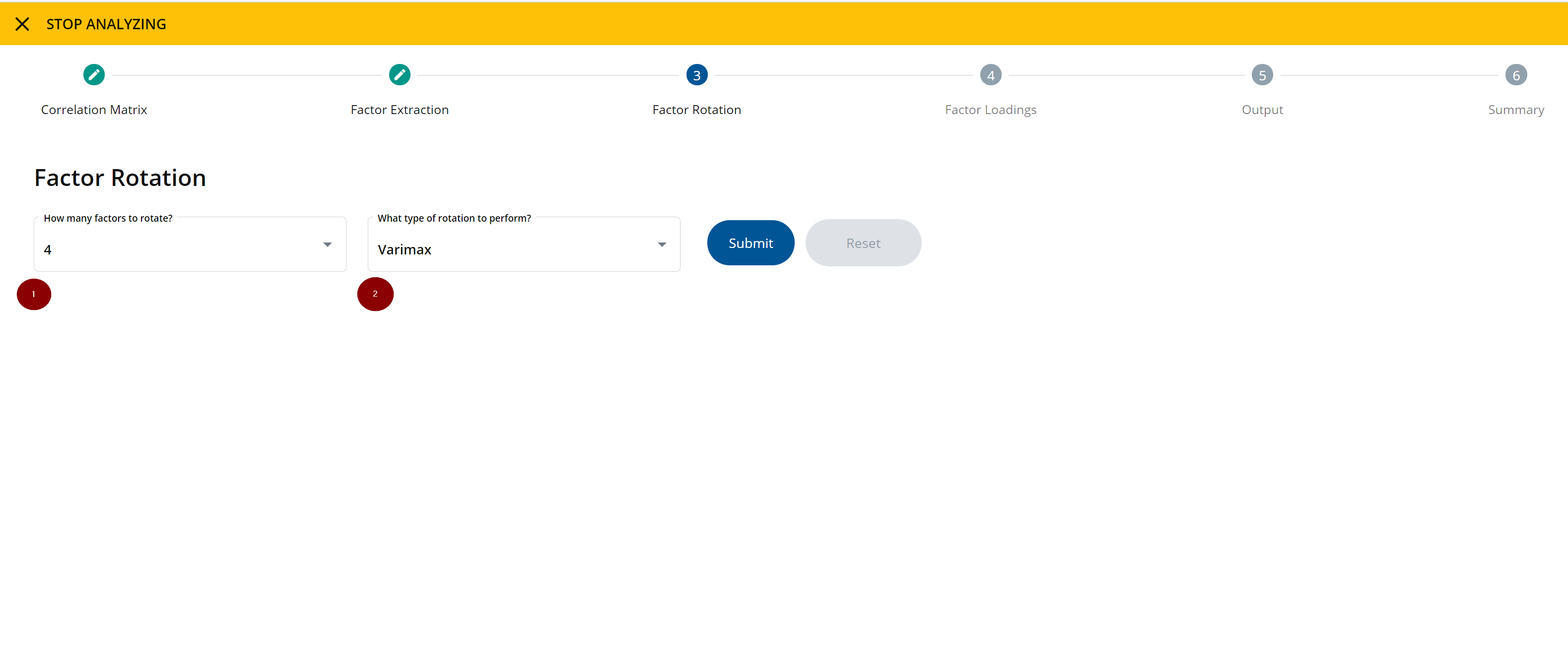
Based on your analysis in step 2, select how many factors you would like to rotate, and select that option in the drop-down menu.
Next, decide which type of rotation to perform: varimax rotation or hand rotation. Varimax and hand rotation are complementary systems with opposing strengths.
Varimax focuses on the mathematically superior solution, ensuring that the factors explain the maximum amount of study variance. The goal is to associate each variable to at most one factor. It rotates all the factors as a group, and focuses on the largest group of the data. Varimax ignores the substantive reality of factors in that it does not care about different groups. For example, if you used a varimax rotation, you would not be able to isolate a particular group of q-sorts, especially if that group is small. If you want to focus on a few q-sorts among the many, you should use hand rotation.
Hand rotation focuses on the theoretically superior solution. It makes possible a factor solution that might more accurately reflect the reality of a particular situation. For example, if you wanted to focus on a few particular q-sorts in a specific demographic, you can use hand rotation to more accurately reflect that group. A hand rotation can isolate individual q-sorts. It provides information such as: “here is a factor that shows me the viewpoint of x.” To conduct a hand rotation, follow these steps:
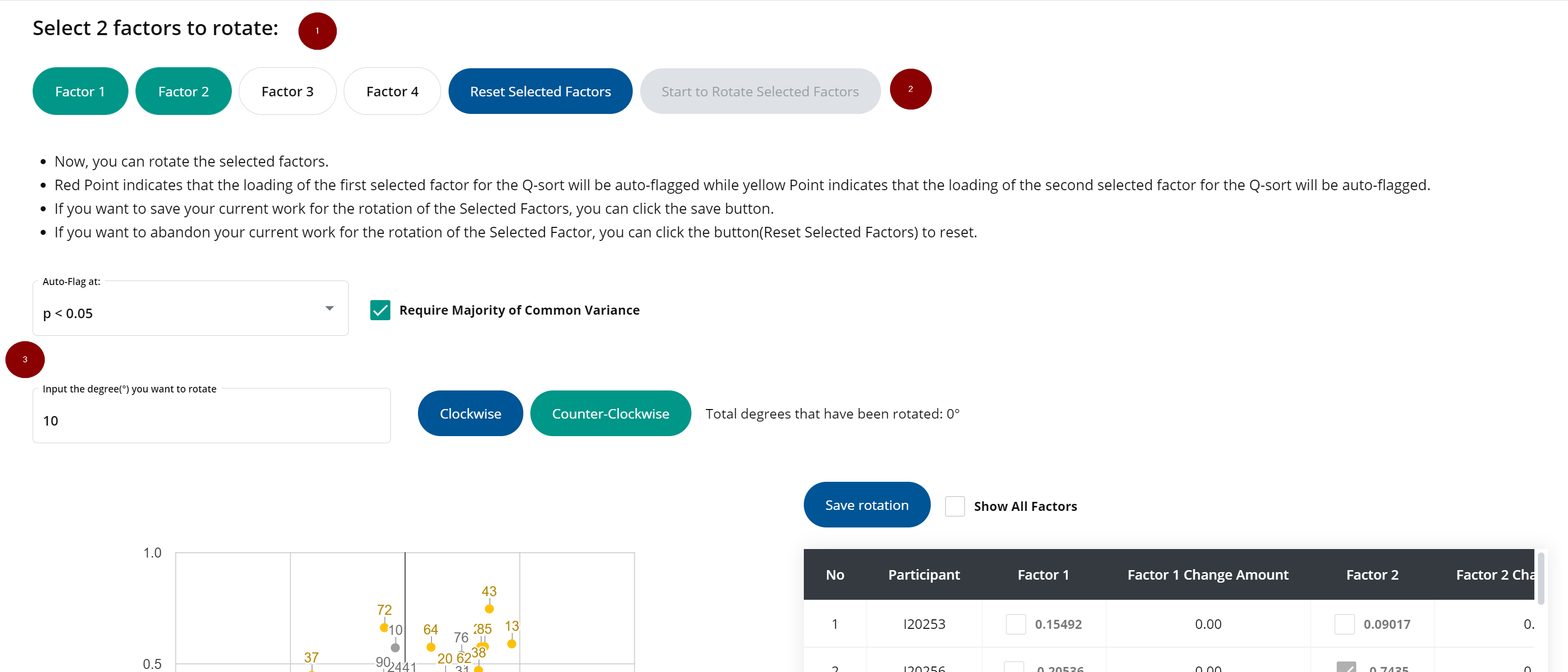
If you select hand rotation, you must first select two factors to rotate.
Next, decide where each factor should ultimately be positioned. The position of the factors may be based on a priori theories or knowledge, or based on your own observations of the data. When you have decided which factors to rotate by hand, press start to rotate selected factors.
A graph will be generated to manually rotate the chosen factors. You are able to rotate either clockwise or counter-clockwise. To rotate the factors, input the degree you want to rotate the factors and then press either clockwise or counter-clockwise.
The graph will be updated in real time, and you will be able to see the degree of rotation (i.e. “Total degrees that have been rotated: 11 degrees”).
Tip
You can contiously click clockwise or counter-clockwire to gradually rotate the graph.
At the bottom of the screen, a table is generated to outline the changes in factor loadings. You may decide to compare it to all other factors, which can be done by pressing “Show All Factors”.
To save the rotation, press “Save Rotation”.
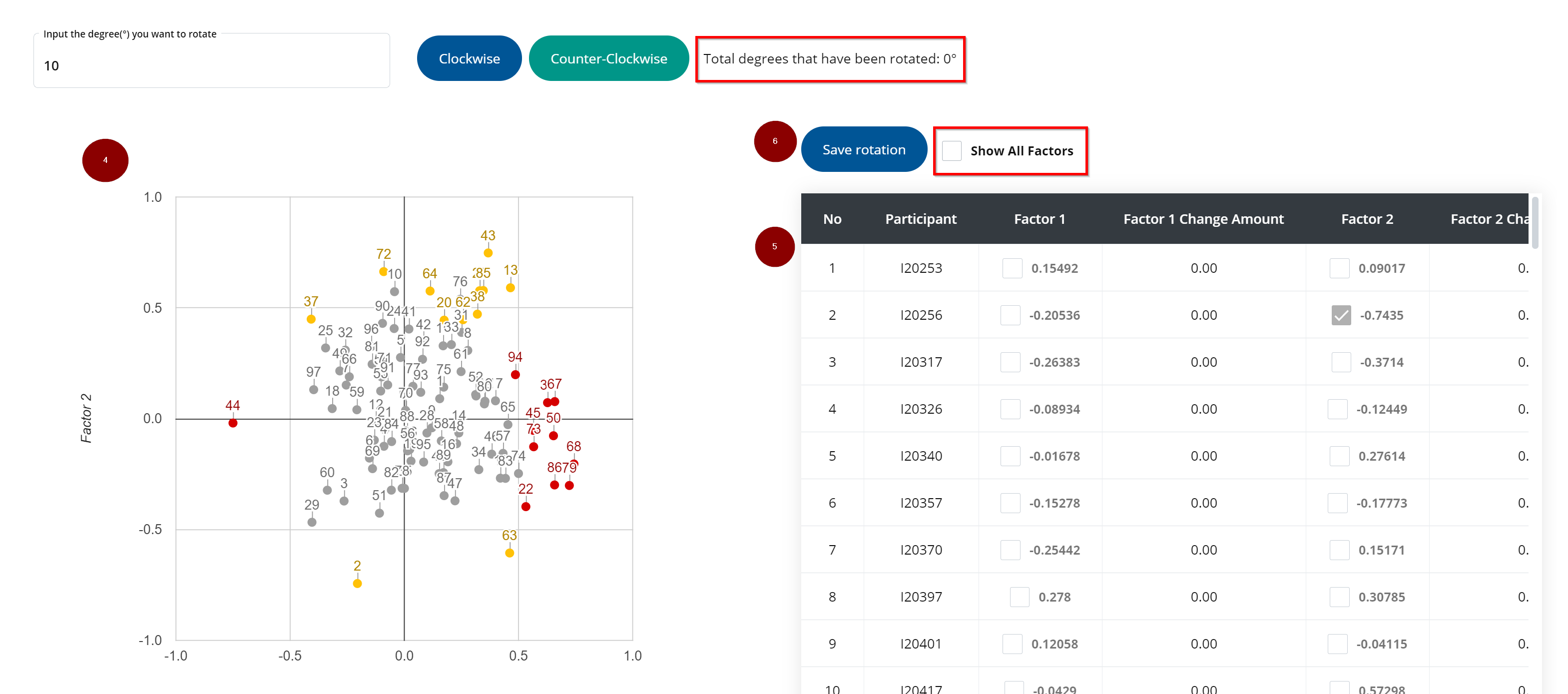
- After you have chosen the factor rotation, press submit. This will bring you to step 4.
Step 3.4: Factor Loadings
This step displays the rotated factor loadings, which are based on previous configurations. The factor loadings (sometimes called “saturations”) provide a measure of the extent to which each q-sort can be said to exemplify a particular factor.
Q Method Software automatically flags significant factor loadings to maximize efficiency.
If you want to look at one particular q-sort, click the menu option located at the end of the row of the specific q-sort. A window containing the single q-sort will pop up, and you are able to look through other q-sorts.
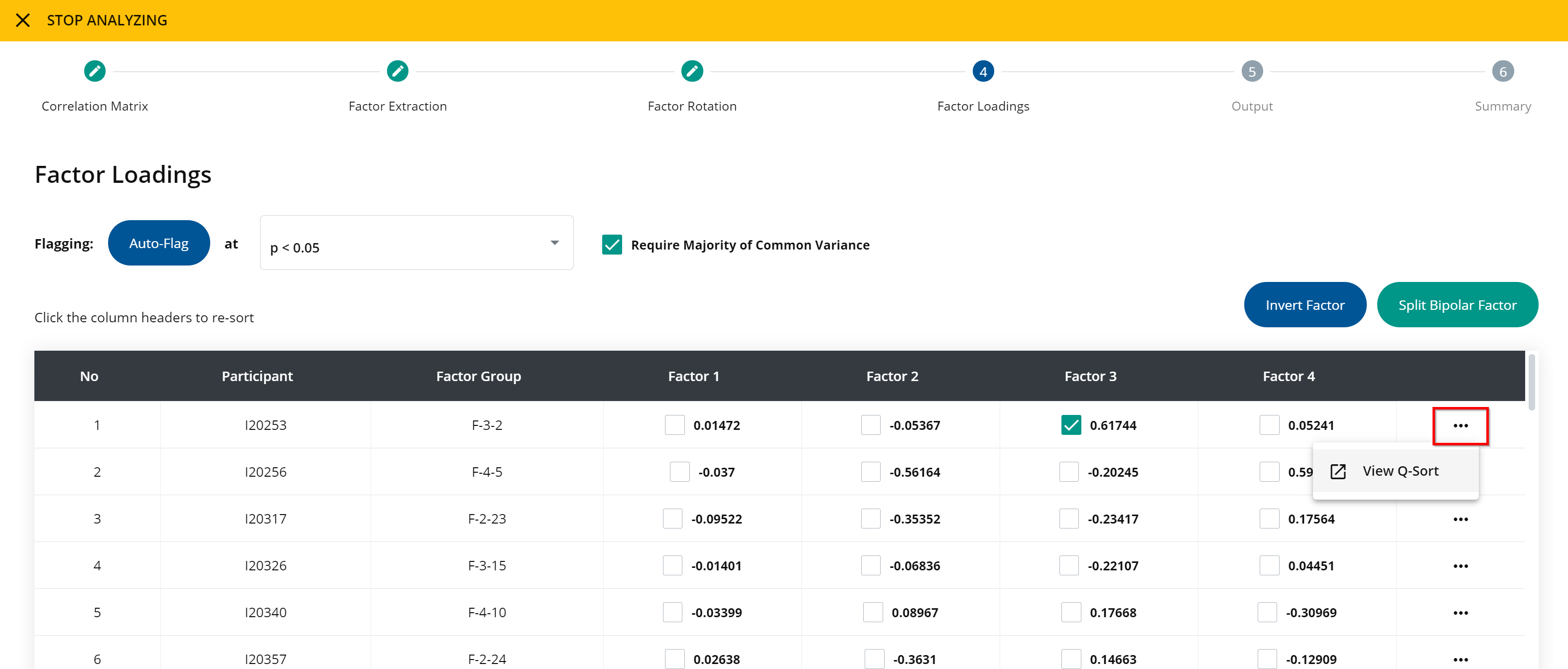
If you included a survey in your study, you may view individual survey responses by clicking the view survey menu item located at the end of each row.
Note
If you do not have a survey in your study, the view survey menu item will not appear.
You can press the button Require Majority of Common Variance to ensure that each q-sort only loads onto one factor significantly. If you deselect this, you might find q-sorts that significantly load on more than one factor.
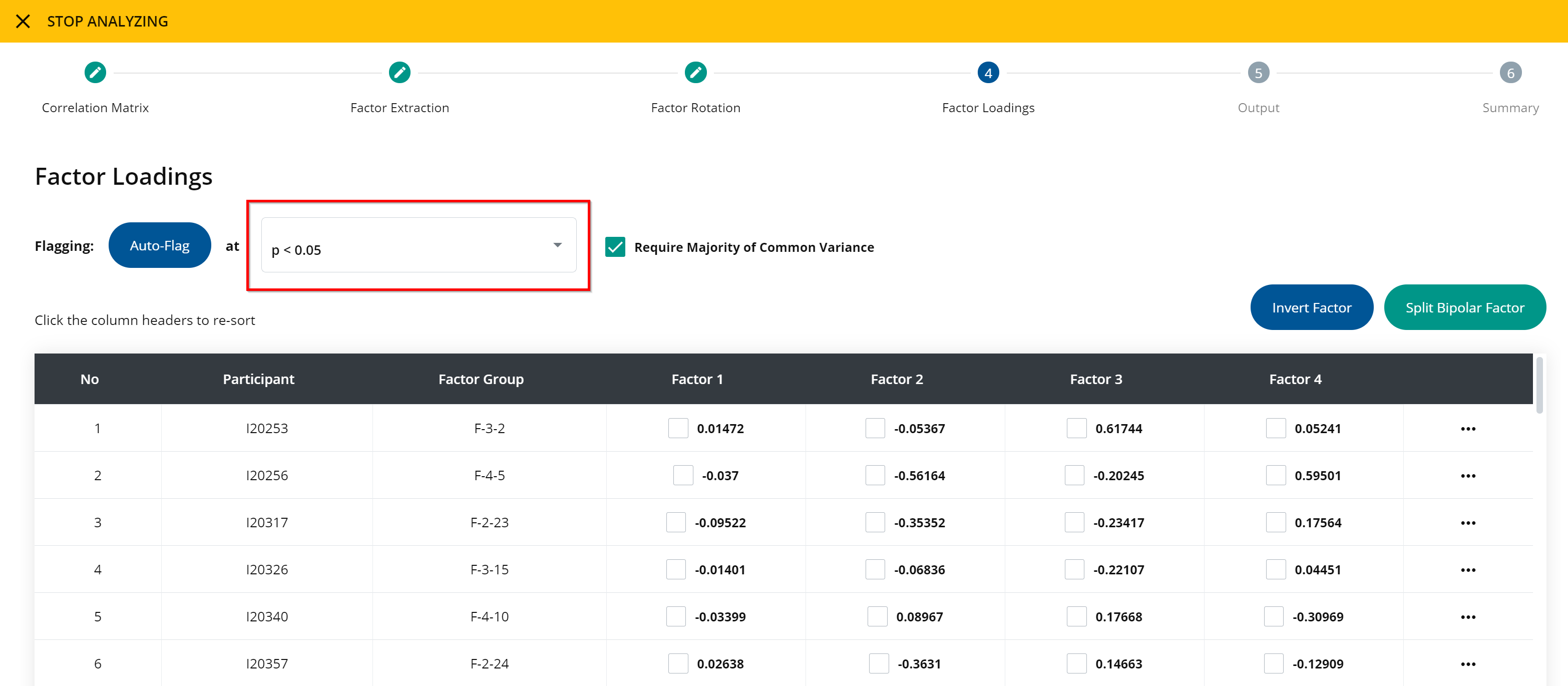
You may also decide to either invert a factor and/or split a bipolar factor. Sometimes when factors are rotated, the factor loadings become negative coefficients rather than positive. To correctly represent the (positive) viewpoints of that factor, you can invert the factor.
To invert a factor:
- Press invert factor.
- Next, select the factor that you want to invert from the drop-down menu, and press submit. If, for example, you decide to invert factor 1, the table will update to display the inverted factor loadings on factor 1.
To split a bipolar factor:
- Press the split bipolar factor button.
- Next, select the factor that you want to split and then press submit. The table will update to include a split bipolar factor. For example, if factor 1 is bipolar, you can split that factor and the table will outline Factor 1a and Factor 1b (representing polar opposite factor loadings).
Tip
If you want to undo a step (invert factor or split bipolar factor), scroll to the bottom of the page. You should find your Action History that outlines any changes you have made to the data. You may click Undo Last Action to delete the last change you made to the data.
You should go through each factor loading and select only the q-sorts that you want to represent in your final array. You might find confounded factor loadings, whereby one q-sort loads significantly on two or more factors. In this case, researchers usually do not associate the particular q-sort with any factor. You might also find non-significant factor loadings.
If you find either a confounded factor loading or a non-significant factor loading, simply deselect the factor loading.
Hyperplane percent by factor
Hyperplane percentages may help you decide whether your chosen rotation method has caused the rotated factor loadings to rotate away from or closer to the optimal solution. The aim of a good rotation result tends to emphasize maximizing the number of near-zero loadings; hyperplane percentages can help you identify whether this aim has been achieved. An optimal solution generally has the following qualities:
- Across each row, there should be one high factor loading and numerous low factor loadings.
- Each column (of factors) should contain only a few high factor loadings and numerous low factor loadings. For every pair of (factor) columns, there should be numerous rows with very low factor loadings on both, and, ideally, one high factor loading.
You can identify which rotation method is ideal for a specific factor analysis case by comparing the hyperplane percentages of the different rotated factor loadings. There are a few ways to do this:
If you have used varimax rotation and then find that the hyperplane count is too small, you might decide to return to step 3.3 to try hand rotation instead.
If you have used hand rotation and then find that the hyperplane count is too small, it may indicate that you either need to modify the hand rotation in step 3.3, or change the rotation from hand rotation to varimax rotation.
After completing the report, you can compare the hyperplane percentages of two separate reports to determine which rotation method yields the higher hyperplane percentage. To do this, follow the steps below:
- Go to the Study Analysis Reports page.
- Click the name of the first report you want to compare. The Summary interface will appear.
- Click the accordion tab labeled Factor Loadings, Hyperplane Percentages & Other Information.
- Make note of the total hyperplane percentage for this report and then exit out of the Summary interface.
- Follow steps 1-4 for the remaining report(s) to compare.
- Generally, the greatest hyperplane percentage indicates a better simple structure.
Tip
If you decide to modify the rotation method, you can make note of the different hyperplane percentages in the notes tab to keep track of the changes.
At the bottom of the page, you can click Show Covariance and Communalities. Two tables will appear: one displaying covariance, and the other showing communality.
- Covariance is a measure of variation between two random variables. A large covariance can mean a strong relationship between variables. A positive covariance indicates that two variables tend to move in the same direction, and a negative covariance reveals that two variables tend to move in inverse directions.
- Communality (also called h^2) indicates the proportion of variance in the responses to the statement which is explained by the identified factors. This common variance ranges between 0 and 1: values closer to 1 indicate that extracted factors may explain more of the variance of an individual item.
Tip
You can use the Notes section to write down any information you want to reference later (i.e. if you have confounding factors in this analysis).
Step 3.5: Output
This step shows the correlations between the factors that you have decided to rotate.
You can also find factor characteristics such as:
- Number of defining variables
- Average relative coefficient
- Composite reliability
- Standard error of factor Z-scores
At the bottom of the page, you will find a composite Q-sort for each factor that has been rotated. This Q-sort represents the ideal Q-sort for each factor.
Step 3.6: Summary
In this step, you will see a summary of the following information:
- Correlation matrix & factor information
- Scree plot & factor rotations
- Factor loadings, hyperplane percentages & other information
- Composite q-sorts & distinguishing statements
Step 3.7: Complete
Press Save to complete the analysis report.
After you have saved and completed the analysis report, you will be redirected to the Study Analysis Reports page. There, you will be able to view the report that you have just completed, in addition to any other reports conducted for your particular study.
Report Summary
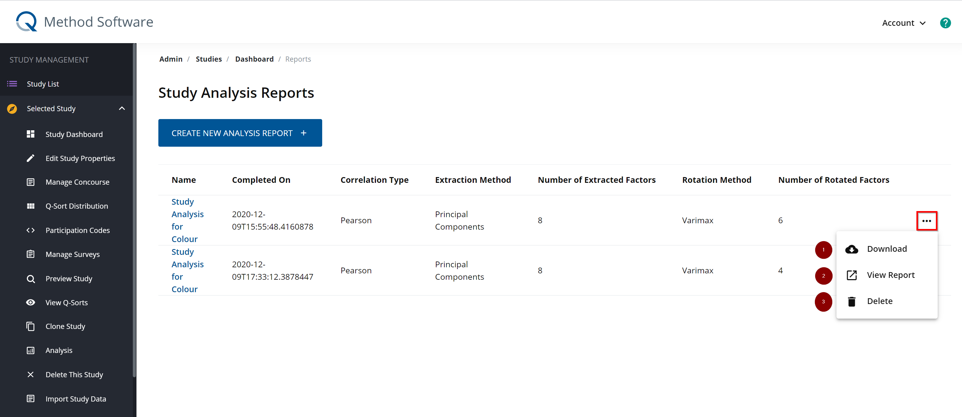
By clicking on the Name of the study, you will be able to view the Summary component of the analysis report (see Step 3.6). You can reference any notes made throughout the report by clicking on the Notes button.
Download Report
You may decide to download the report by clicking on Download Report.